Introduction
GPS measurements in real-world drone navigation have 2-5m of error. If you base your control directly on raw GPS measurements, the controls will not be smooth. The drone’s controller ends up fighting measurement noise instead of actual disturbances.
Kalman filter can address this problem. The filter fuses noisy GPS position measurements with clean IMU acceleration data to produce smooth state estimates. The result: 62.8% reduction in position error compared to raw GPS measurements.
The Problem: Sensor-Model Tension
The fundamental challenge in state estimation is the tension between two imperfect sources of information.
Sensors are inherently imperfect. Measurements can be noisy, biased, incomplete, or disrupted by environmental factors. They capture what’s happening now but don’t predict future state or account for underlying dynamics. GPS, for example, provides position measurements but with significant noise (±3m standard deviation). Computing velocity from GPS using numerical derivatives amplifies this noise dramatically.
Physics models are mathematical representations based on physical laws. They are deterministic or probabilistic frameworks that integrate prior knowledge. Their limitation is that they’re abstractions - often simplified to make computation feasible. They may ignore real-world complexities like wind, drag, or sensor biases. Over time, model predictions can drift from reality.
The fundamental tension arises from this dichotomy. Sensors provide ground truth obstructed by uncertainty, while physics models offer coherent predictions that can diverge from reality due to idealizations.
Consider a concrete example from my implementation: GPS says “you’re at 10.3m altitude” (noisy but real), while the physics model says “based on last position and IMU acceleration, you should be at 9.8m” (smooth but possibly drifting). Which do you trust? Trust GPS too much and you get jerky control. Trust the model too much and you drift away from reality.
The outcome is a trade-off in trust between these two sources.
Why This Matters for Control Systems
I previously implemented PID controllers for waypoint navigation. When you feed noisy measurements into a PID controller:
- The derivative term (Kd) amplifies noise. If GPS jumps ±3m, the velocity estimate oscillates wildly, causing the drone to fight phantom movements.
- The integral term (Ki) accumulates these noisy errors over time.
- The controller is essentially fighting measurement noise instead of actual disturbances like wind.
Without filtering, your PID controller cannot distinguish between real state changes and sensor noise. This is unacceptable for stable autonomous flight.
The Solution: Kalman Filtering
The Kalman filter solves this problem by computing the optimal balance between prediction and measurement automatically. It’s a two-step recursive algorithm that runs continuously during flight.
The Two-Step Cycle
1. Predict Step (runs at 100 Hz using IMU acceleration)
The filter uses a physics model to predict where the drone should be at the next timestep:
x_p = A × x + B × uP_p = A × P × A^T + QWhere:
x_pis the predicted state [position, velocity]Ais the state transition matrix (constant velocity model)Bis the control input matrix (acceleration from IMU)uis the control input (acceleration)P_pis the predicted covariance (uncertainty)Qis the process noise (model uncertainty)
Uncertainty grows during this step because our physics model is imperfect. We add process noise Q to account for unmodeled dynamics.
2. Correct Step (runs at 10 Hz when GPS measurement arrives)
When a GPS measurement arrives, the filter compares it with the prediction and updates its belief:
y = z - H × x_p # Innovation (measurement - prediction)S = H × P_p × H^T + R # Innovation covarianceK = P_p × H^T × S^(-1) # Kalman gainx = x_p + K × y # Update stateP = P_p - K × H × P_p # Update covarianceWhere:
zis the GPS measurementHis the measurement matrix (we measure position, not velocity)Kis the Kalman gain (optimal weight)Ris the measurement noise covariance
Uncertainty shrinks during this step because the measurement provides new information.
The Kalman Gain: Optimal Weighting
The Kalman gain K is the most important concept in the filter. It automatically computes the optimal trust balance between prediction and measurement.
When K is close to 1, our certainty about the measurement grows. We trust the sensor more because our prediction is uncertain (large P_p) or the sensor is reliable (small R).
When K is close to 0, we’re more certain about the physical model. We trust the prediction more because our model is confident (small P_p) or the sensor is noisy (large R).
The filter adjusts K dynamically based on the relative uncertainties. No manual tuning required - the mathematics finds the optimal weight that minimizes mean squared error.
Implementation Details
State Representation
I chose a 2D state vector:
x = [position, velocity]^TWhy include velocity? GPS only provides position. Computing velocity from GPS using numerical derivatives is very noisy. The Kalman filter estimates velocity as a “hidden state” - we don’t measure it directly, but infer it from how position changes over time. This gives us smooth velocity estimates for free, which is crucial for control.
The Matrices
State Transition Matrix A (constant velocity model):
A = [[1, dt], [0, 1]]This represents Newton’s first law: objects in motion stay in motion at constant velocity. The matrix implements:
new_position = old_position + velocity × dtnew_velocity = old_velocity
Velocity doesn’t change unless we apply acceleration (control input u).
Control Input Matrix B:
B = [[0.5 × dt²], [dt ]]This maps IMU acceleration to state changes using kinematic equations:
position += 0.5 × acceleration × dt²velocity += acceleration × dt
Measurement Matrix H:
H = [[1, 0]]This specifies what we can measure. H = [1, 0] means “I can measure position but NOT velocity.” When we compute z = H @ x, we get:
z = [1, 0] @ [position, velocity] = positionGPS gives us position directly. We have to estimate velocity from how position changes.
Process Noise Covariance Q:
q = process_noise²Q = q × [[dt⁴/4, dt³/2], [dt³/2, dt² ]]This represents uncertainty in the physics model. Process noise grows proportionally to time passed. The specific structure comes from the discrete-time white noise acceleration model. I used process_noise = 0.5 based on expected model inaccuracies.
Measurement Noise Covariance R:
R = [[9.0]] # GPS variance (3m std dev)This represents sensor noise variance. For GPS with 3m standard deviation, R = 3² = 9. If we set R too high, the filter focuses too much on the physical model and ignores measurements. If R is too low, the filter trusts noisy measurements too much. There has to be some balance - the optimal balance comes from accurate characterization of actual sensor noise.
Results
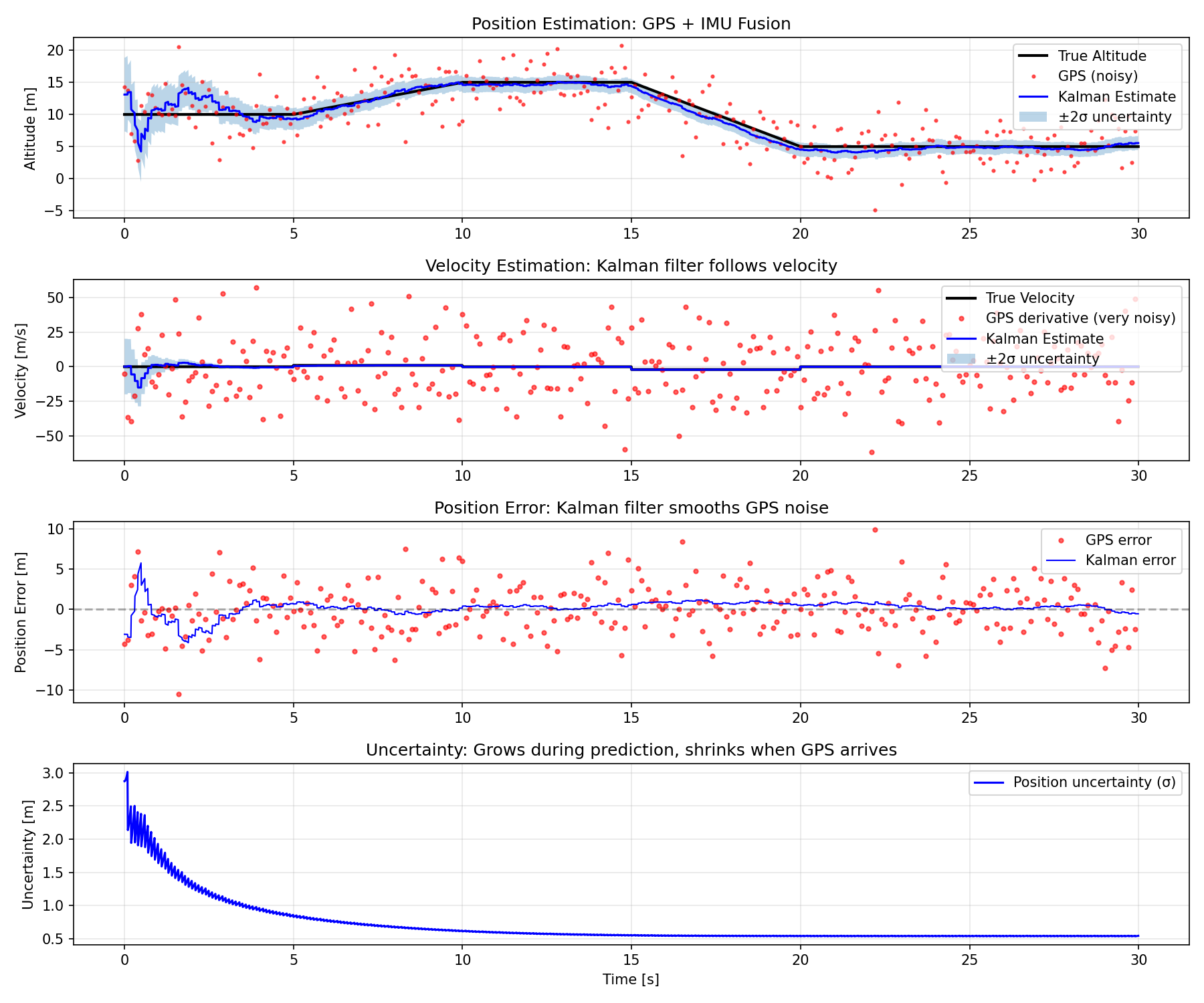
I tested the implementation on a simulated vertical motion scenario:
- Drone hovers at 10m, climbs to 15m, descends to 5m
- GPS provides noisy measurements (±3m error) at 10 Hz
- IMU provides acceleration at 100 Hz
- Simulation runs for 30 seconds
Quantitative Performance
Position Error (Raw GPS): 2.648 m RMSPosition Error (Kalman): 0.984 m RMSImprovement: 62.8%The filter successfully reduced position error by nearly two-thirds compared to raw GPS measurements.
Qualitative Observations
Position tracking: The Kalman estimate is smooth and tracks the true trajectory closely. It doesn’t jump around like raw GPS. Between GPS updates, the filter uses IMU acceleration to predict position, resulting in 100 Hz state updates even though GPS only arrives at 10 Hz.
Velocity estimation: The filter produces clean velocity estimates. Computing velocity from GPS using numerical derivatives is extremely noisy - the raw GPS derivative has ~10x more noise than the Kalman estimate. This smooth velocity is essential for stable control.
Uncertainty behavior: The covariance P oscillates as expected. It grows during prediction steps (model uncertainty accumulates) and shrinks when GPS measurements arrive (new information reduces uncertainty). This oscillation pattern validates that the filter is working correctly.
Applications
This algorithm is not theoretical. It’s the backbone of autonomous systems:
Flight controllers: ArduPilot and PX4 use Extended Kalman Filters (EKF) for state estimation. They fuse GPS, IMU, magnetometer, barometer, and optical flow to estimate position, velocity, and attitude. My 1D implementation is a simplified version of what runs on every commercial drone.
GPS receivers: Your phone uses Kalman filtering to combine satellite signals with motion models (from accelerometer and gyroscope) to produce smooth position estimates.
Autonomous vehicles: Tesla and other self-driving systems use variants of Kalman filtering for sensor fusion, combining radar, lidar, camera, and IMU data.
This approach is the standard when you have multiple imperfect information sources that need to be combined optimally.
Next Steps
This project establishes a foundation for more advanced work:
Integrate with PID controller: Use Kalman-filtered estimates instead of raw GPS in the cascaded PID controller. Expected result: smoother control with less oscillation.
Extend to 3D position: Currently the filter estimates 1D altitude. Extending to 3D position estimation requires a 6D state: [x, y, z, vx, vy, vz]. The mathematics remain the same, just with larger matrices.
Extended Kalman Filter (EKF): The current implementation assumes linear dynamics. Real quadrotors have nonlinear dynamics (rotation matrices, attitude kinematics). EKF linearizes the dynamics around the current estimate.
Multi-sensor fusion: Add barometer for altitude, magnetometer for heading. Each sensor has different noise characteristics and update rates. Kalman filtering handles this naturally.
Conclusion
Implementing a Kalman filter from scratch provided deep insight into optimal estimation and sensor fusion. The fundamental concept - balancing imperfect predictions with noisy measurements - is elegant in its mathematical formulation but requires careful attention to implementation details.
This work is part of a larger learning path toward autonomous systems development for defense applications. Understanding Kalman filtering is foundational - it appears in every serious robotics system, from drones to spacecraft.
References
- Kalman, R. E. (1960). “A New Approach to Linear Filtering and Prediction Problems”
- Welch, G., & Bishop, G. “An Introduction to the Kalman Filter” (UNC-Chapel Hill TR)
- Labbe, R. “Kalman and Bayesian Filters in Python” (online textbook)
- ArduPilot EKF documentation: ardupilot.org/dev/docs/extended-kalman-filter.html