Recursive Filters: SMA, EMA, Low‑Pass, and a Tiny Kalman

While exploring optimizers I fell down the rabbit hole of recursive filters. This post is a compact, practical tour of smoothers you can use when measurements are noisy but latency and compute are tight. We’ll keep the math minimal, the intuition high, and focus on when and why to use SMA, EMA/low‑pass, and a tiny 1D Kalman.

If you are here just for code, my Kaggle Notebook can be found here.

Why recursive filters

Recursive filters shine when compute and memory are scarce, or when data arrives as a stream and you must react immediately.

• O(1) memory: you keep just the last state (and maybe a running sum) rather than a long buffer.
• O(1) compute per sample: one or two multiply‑adds per step—perfect for microcontrollers and tight loops.
• Online, low‑latency: produce an updated estimate as soon as a sample arrives; no need to wait for a full window.
• Simple, robust implementations: easy to port, vectorize, or run in reduced precision.
• Graceful with irregular sampling: updates are incremental and don’t assume batch availability.

Intuition note

Recursive filters that we’ll use, all use constant‑size state. That’s why they’re common in embedded systems, robotics control loops, mobile sensor smoothing and telemetry.

Notation

• $x_t$: the raw observation at time step $t$.
• $s_t$: the smoothed estimate at time $t$.
• $k$: window size (for moving averages).
• $\alpha\in[0,1]$: smoothing factor (higher $\alpha$ = smoother, but laggier).

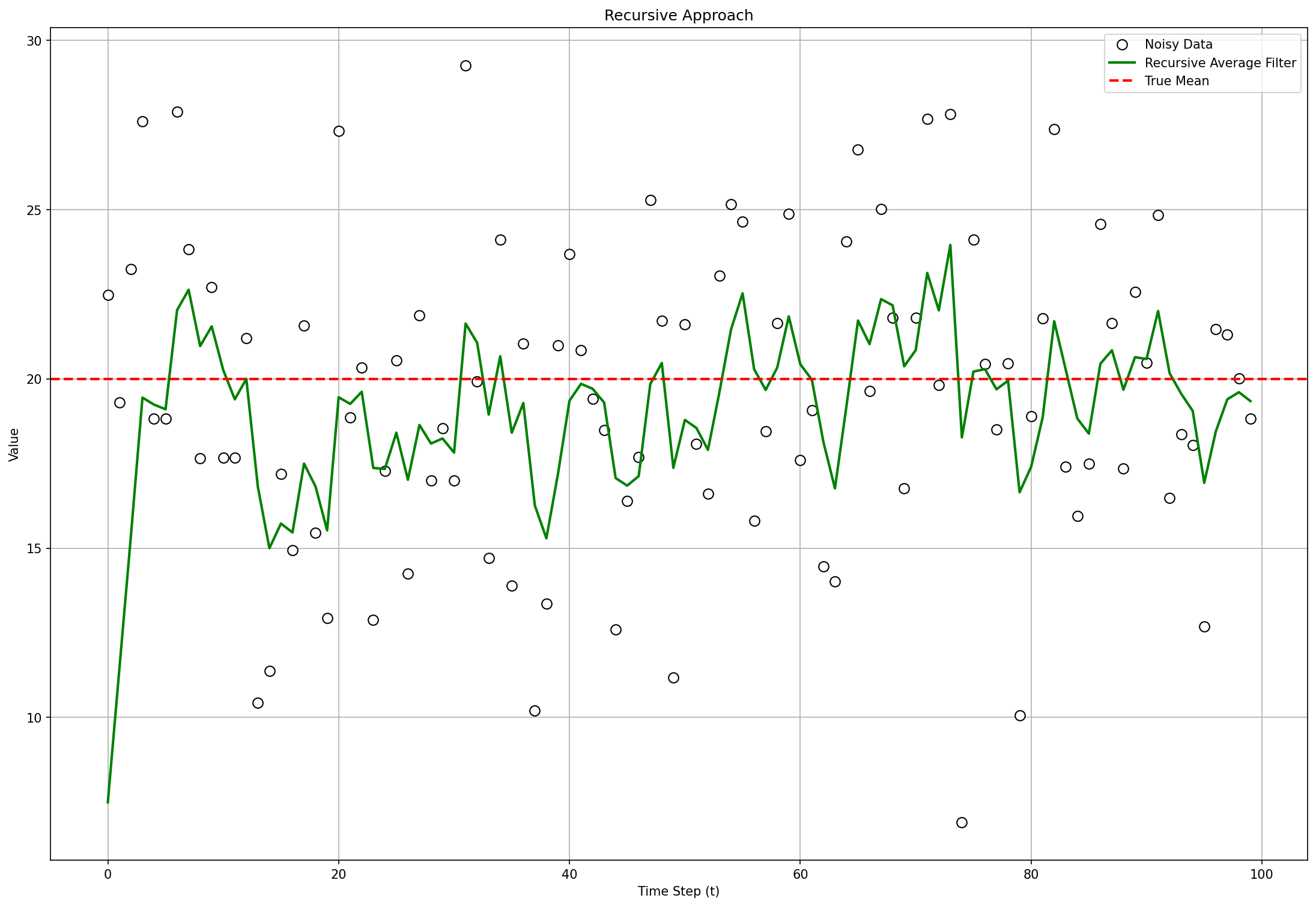
Recursive Average Filter (also known as EMA)

The one‑liner you’ll use most:

$$s_t = \alpha\, s_{t-1} + (1-\alpha)\, x_t.$$

Many libraries choose $\alpha$ directly; our example consists of $k$ data points and we define alpha as $\alpha = \tfrac{k-1}{k}$ to make notation easier to hold in our memory.

Intuition note

This behaves like a leaky integrator. Bigger $\alpha$ forgets the past more slowly (smoother, more lag). The initial line takes a few iterations before it can get closer to the real mean value.

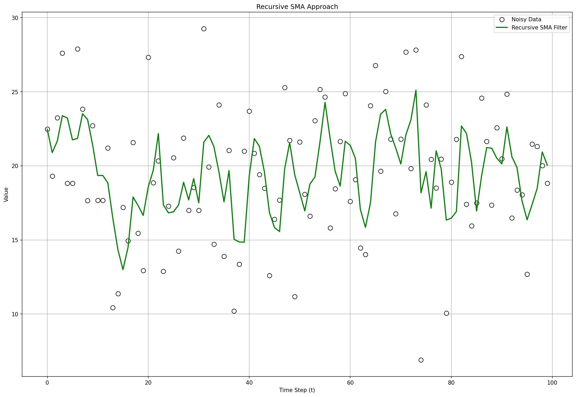
Simple Moving Average (SMA)

Windowed average over the last $k$ samples:

$$s_t = \frac{1}{k} \sum_{i=0}^{k-1} x_{t-i}.$$

Intuition note

Great at crushing noise, but it lags and needs a buffer of the last $k$ points. Spikes are “diluted” equally across the window.

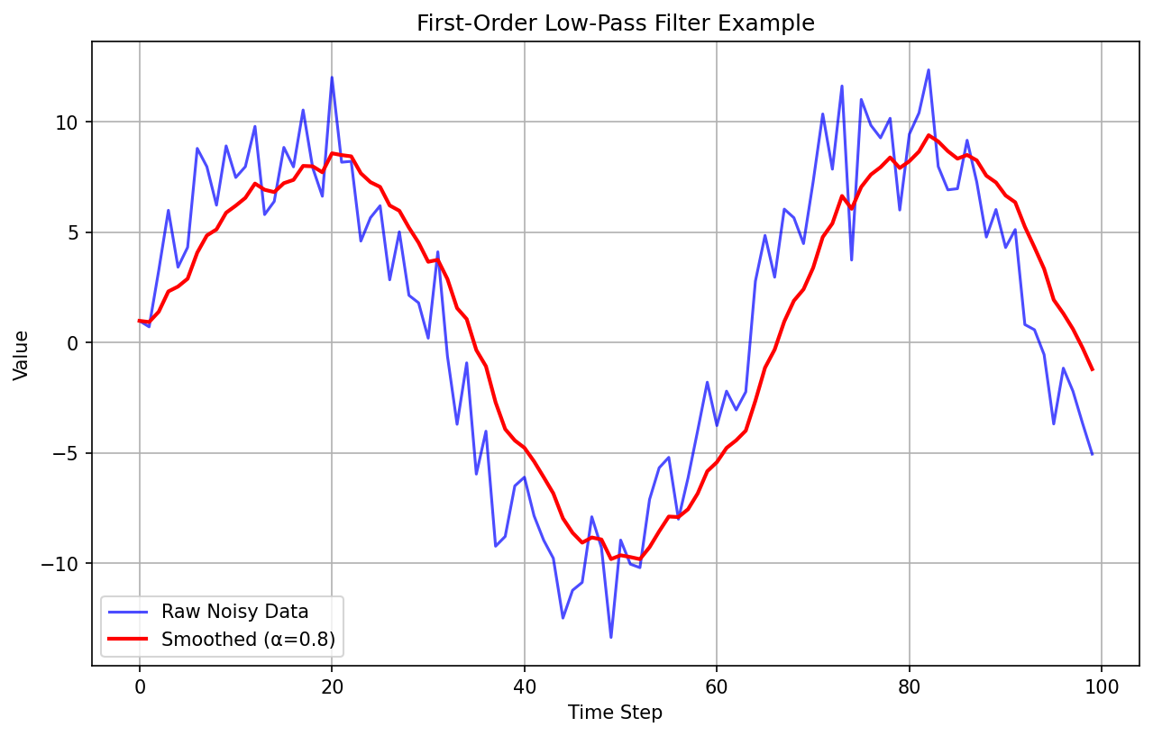
First‑Order Low‑Pass Filter

In discrete time, the classic low‑pass is algebraically the same as the EMA:

$$y_t = \alpha\, y_{t-1} + (1-\alpha)\, x_t.$$

Different name, same form. You pick $\alpha$ to trade off noise suppression versus responsiveness.

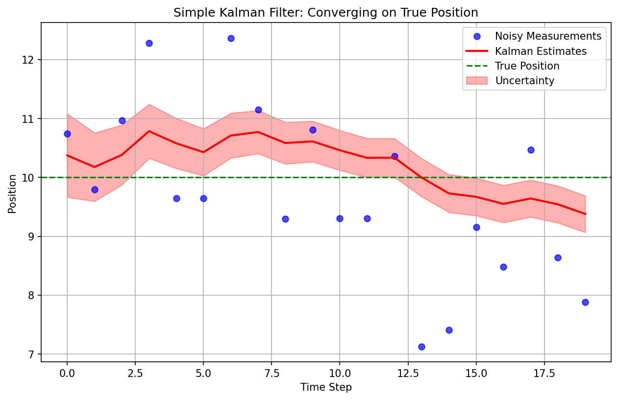
A Tiny 1D Kalman Update

This is just scratching the surface of a Kalman Filter - a tiny 1D Kalman Update. This is my first attempt at building intuition before I can jump to an actual KF.

When you know your sensor noise ($R$) and process noise ($Q$), Kalman gives you an adaptive gain that automatically balances trust between the prediction and the measurement. For a constant‑value model ($A=H=1$):

Predict:

$$\hat{x}_t^{-} = \hat{x}_{t-1},\quad P_t^{-} = P_{t-1} + Q.$$

Update:

$$K_t = \frac{P_t^{-}}{P_t^{-} + R},\quad \hat{x}_t = \hat{x}_t^{-} + K_t\,(z_t - \hat{x}_t^{-}),\quad P_t = (1 - K_t) P_t^{-}.$$

Intuition note

If measurements are noisy (large $R$), $K_t$ shrinks and you trust the prior more. If the process is volatile (large $Q$), $P_t^{-}$ grows and $K_t$ increases—trust the new measurement more.

Choosing parameters

• SMA window $k$: larger $k$ = smoother but laggier. Needs a buffer.
• EMA/low‑pass $\alpha$: start around $0.8$–$0.95$. Tune by eyeballing lag vs. noise.
• Kalman $(Q, R)$: set $R$ to your sensor variance; set $Q$ to how much you expect the latent to drift between steps.

What next?

SMA is simple and robust; EMA/low‑pass is the default for streaming; and a tiny Kalman filter adds principled adaptivity when you can estimate noise. Two first filters are easy to implement, Kalman though was simplied to its 1D version. An actual Kalman Filter is way more complicated and it should be the subject of my future learning. Hopefully there will be a text about it of a decent quality.

Standing on the shoulders of giants

Resource that I used:

• Dr. Shane Ross videos on the topic
• Kalman Filter explained simply